Seaborn은 Matplotlib의 기능과 스타일을 확장한 파이썬 시각화 도구의 고급 버전이다.
데이터셋 가져오기
titanic 데이터셋을 가져와보자.
import seaborn as sns

titanic = sns.load_dataset('titanic')

print(titanic.head())
print('\n')
print(titanic.info())

   survived  pclass     sex   age  sibsp  parch     fare embarked  class  \
0         0       3    male  22.0      1      0   7.2500        S  Third
1         1       1  female  38.0      1      0  71.2833        C  First
2         1       3  female  26.0      0      0   7.9250        S  Third
3         1       1  female  35.0      1      0  53.1000        S  First
4         0       3    male  35.0      0      0   8.0500        S  Third

     who  adult_male deck  embark_town alive  alone
0    man        True  NaN  Southampton    no  False
1  woman       False    C    Cherbourg   yes  False
2  woman       False  NaN  Southampton   yes   True
3  woman       False    C  Southampton   yes  False
4    man        True  NaN  Southampton    no   True


<class 'pandas.core.frame.DataFrame'>
RangeIndex: 891 entries, 0 to 890
Data columns (total 15 columns):
 #   Column       Non-Null Count  Dtype
---  ------       --------------  -----
 0   survived     891 non-null    int64
 1   pclass       891 non-null    int64
 2   sex          891 non-null    object
 3   age          714 non-null    float64
 4   sibsp        891 non-null    int64
 5   parch        891 non-null    int64
 6   fare         891 non-null    float64
 7   embarked     889 non-null    object
 8   class        891 non-null    category
 9   who          891 non-null    object
 10  adult_male   891 non-null    bool
 11  deck         203 non-null    category
 12  embark_town  889 non-null    object
 13  alive        891 non-null    object
 14  alone        891 non-null    bool
dtypes: bool(2), category(2), float64(2), int64(4), object(5)
memory usage: 80.7+ KB
None
회귀선이 있는 산점도
regplot() 함수는 서로 다른 2개의 연속 변수 사이의 산점도를 그리고 선형회귀분석에 의한 회귀선을 같이 나타낸다
import matplotlib.pyplot as plt

titanic = sns.load_dataset('titanic')


sns.set_style('darkgrid')

fig=plt.figure(figsize=(15, 5))
ax1 = fig.add_subplot(1,2,1)
ax2 = fig.add_subplot(1,2,2)

sns.regplot(x = 'age',
			y = 'fare',
            data = titanic,
            ax = ax1)

sns.regplot(x = 'age',
			y = 'fare',
            data = titanic,
            ax = ax2,
            fig_reg = False) #회귀선 미표시 옵션

plt.show()
히스토그램 / 커널 밀도 그래프
커널 밀도 그래프는 밀도 분포 함수이고, 단일 변수의 데이터 분포를 확인할 때 distplot() 함수를 이용한다.
기본값으로 히스토그램과 커널 밀도 함수를 그래프로 출력한다.
fig = plt.figure(figsize=(15,5))
ax1 = fig.add_subplot(1,3,1)
ax2 = fig.add_subplot(1,3,2)
ax3 = fig.add_subplot(1,3,3)

sns.displot(titanic['fare'], ax=ax1)

sns.distplot(titanic['fare'], hist=False, ax=ax2) #히스토그램 표시 X

sns.distplot(titanic['fare'], kde=False, ax=ax3) #커널 함수 표시 X

ax1.set_title('titanic fare - hist/ked')
ax2.set_title('titanic fare - ked')
ax3.set_title('titanic fare - hist')

plt.show()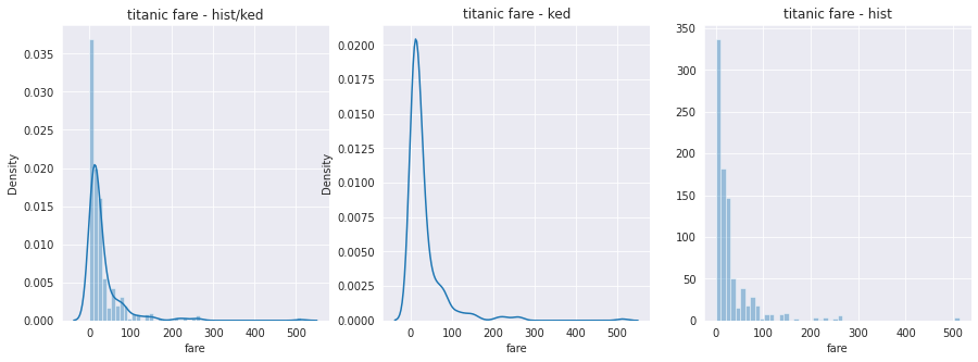
히트맵
heatmap() 메소드는 2개의 범주형 변수를 각각 x, y축에 놓고 데이터를 매트릭스 형태로 분류한다.
#피봇 테이블 생성
table = titanic.pivot_table(index=['sex'], columns=['class'], aggfunc='size')


sns.heatmap(table,
			annot=True, fmt='d', #데이터 값 표시 여부, 정수형 포맷
            cmap='YlGnBu',		 #컬러맵
            linewidth=.5,		 #구분선
            cbar=False)			 #컬러바 표시 여부

plt.show()
범주형 데이터의 산점도
범주형 변수에 들어있는 각 범주별 데이터의 분포를 확인할 수 있다.
stripplot() 함수와 swarmplot() 함수를 사용할 수 있다,
swarmplot() 함수는 데이터의 분산까지 고려하여, 데이터 포인트가 서로 중복되지 않도록 그림을 그린다.
sns.set_style('whitegrid')

fig = plt.figure(figsize=(15, 5))
ax1 = fig.add_subplot(1,2,1)
ax2 = fig.add_subplot(1,2,2)

#이산형 변수의 분포 - 데이터 분산 미고려
sns.stripplot(x = 'class',
			  y = 'age',
              data = titanic,
              ax = ax1)

#데이터 분산 고려 (중복 x)
sns.swarmplot(x='class',
			  y='age',
              data = titanic,
              ax = ax2)

ax1.set_title('Strip Plot')
ax2.set_title('Strip Plot')

plt.show()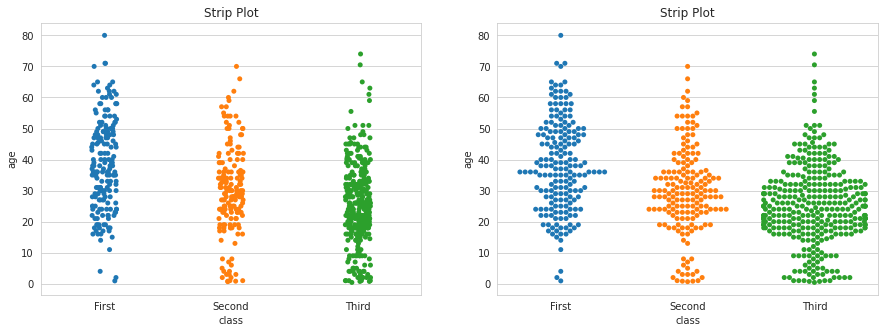
여기에 hue='sex' 옵션을 추가하면, 'sex'열의 데이터 값인 남녀 성별을 색상으로 구분하여 출력한다.
막대 그래프
barplot() 함수를 이용하여 막대그래프를 그릴 수 있다.
fig = plt.figure(figsize=(15, 5))
ax1 = fig.add_subplot(1,3,1)
ax2 = fig.add_subplot(1,3,2)
ax3 = fig.add_subplot(1,3,3)

sns.barplot(x='sex', y='survived', data=titanic, ax=ax1)

#hue 옵션 추가
sns.barplot(x='sex', y='survived', hue='class', data=titanic, ax=ax2)

#dodge=False 설정해서 누적해서 출력한다
sns.barplot(x='sex', y='survived', hue='class', dodge=False, data=titanic, ax=ax3)

ax1.set_title('titanic survived - sex')
ax2.set_title('titanic survived - sex/class')
ax3.set_title('titanic survived - sex/class(stacked)')
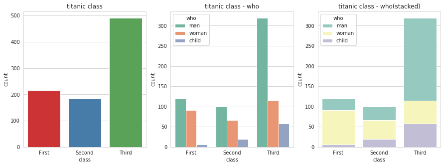
빈도 그래프
각 범주에 속하는 데이터의 개수를 막대 그래프로 나타내는 countplot() 함수가 있다.
fig = plt.figure(figsize=(15,5))
ax1 = fig.add_subplot(1,3,1)
ax2 = fig.add_subplot(1,3,2)
ax3 = fig.add_subplot(1,3,3)

sns.countplot(x='class', palette='Set1', data=titanic, ax=ax1)
#hue 옵션에 who 추가
sns.countplot(x='class', hue='who', palette='Set2', data=titanic, ax=ax2)

#누적으로 쌓기
sns.countplot(x='class', hue='who', palette='Set3', dodge=False, data=titanic, ax=ax3)

ax1.set_title('titanic class')
ax2.set_title('titanic class - who')
ax3.set_title('titanic class - who(stacked)')

plt.show()
박스플룻 / 바이올린 플롯
박스플롯은 boxplot() 함수를 사용하여 범주형 데이터 분포와 주요 통계 지표를 함께 제공한다
그러나 데이터가 퍼져 있는 분산의 정도를 정확히 알기 어려워서, 바이올린 그래프를 함께 그리는 경우가 있다.
바이올린 그래프는 violinplot() 함수로 그린다.
sns.set_style('darkgrid')
fig = plt.figure(figsize=(15,10))

ax1 = fig.add_subplot(2,2,1)
ax2 = fig.add_subplot(2,2,2)
ax3 = fig.add_subplot(2,2,3)
ax4 = fig.add_subplot(2,2,4)

sns.boxplot(x='alive', y='age', data=titanic, ax=ax1)
sns.boxplot(x='alive', y='age', hue='sex', data=titanic, ax=ax2)
sns.violinplot(x='alive', y='age', data=titanic, ax=ax3)
sns.violinplot(x='alive', y='age', hue='sex', data=titanic, ax=ax4)

plt.show()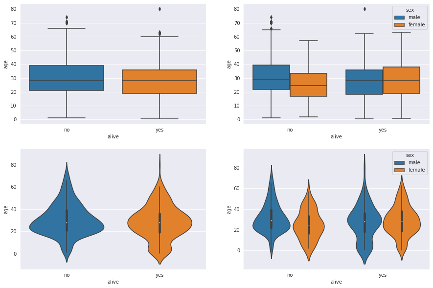
조인트 그래프
jointplot() 함수는 산점도를 기본으로 표시하고, x-y축에 각 변수에 대한 히스토그램을 동시에 보여준다.
두 변수의 관계와 데이터가 분산되어 있는 정도를 한눈에 파악하기 좋다.
sns.set_style('dark')

#산점도(기본값)
j1 = sns.jointplot(x='fare', y='age', data=titanic)

#회귀선
j2 = sns.jointplot(x='fare', y='age', kind='reg', data=titanic)

#육각 그래프
j3 = sns.jointplot(x='fare', y='age', kind='hex', data=titanic)

#커널 밀집 그래프
j4 = sns.jointplot(x='fare', y='age', kind='kde', data=titanic)

j1.fig.suptitle('titanic fare - scatter', size=15)
j2.fig.suptitle('titanic fare - reg', size=15)
j3.fig.suptitle('titanic fare - hex', size=15)
j4.fig.suptitle('titanic fare - kde', size=15)

plt.show()


조건 적용하여 화면 그리드로 분할
FacetGrid() 함수는 행, 열 방향으로 서로 다른 조건을 적용하여 여러 개의 서브 플롯을 만든다.
그리고 각 서브 플롯에 적용할 그래프 종류를 map() 메소드를 이용하여 그리드 객체에 전달한다.
sns.set_style('whitegrid')

#조건에 따라 그리드 나누기
g = sns.FacetGrid(data=titanic, col='who', row='survived')

#그래프 적용하기
g = g.map(plt.hist, 'age')
이변수 데이터의 분포
pairplot() 함수는 인자로 전달되는 데이터프레임의 열(변수)을 두 개씩 짝을 지을 수 있는 모든 조합에 대해 표현한다.
같은 변수끼리 짝을 이루는 대각선 방향으로는 히스토그램을 그리고
서로 다른 변수 간에는 산점도를 그린다.
titanic_pair = [['age', 'pclass', 'fare']]

g = sns.pairplot(titanic_pair)
'Study > 혼자 공부하는 판다스' 카테고리의 다른 글
| 혼자 공부하는 판다스 - 데이터 사전 처리(누락 데이터 처리, 중복 데이터 처리) (0) | 2022.04.22 |
|---|---|
| 혼자 공부하는 판다스 - Folium 라이브러리 (지도 활용) (0) | 2022.04.21 |
| 혼자 공부하는 판다스 - 시각화 도구 (0) | 2022.04.05 |
| 혼자 공부하는 판다스 - 데이터 살펴보기 (0) | 2022.04.04 |
| 혼자 공부하는 판다스 - 데이터 저장하기 (0) | 2022.04.04 |


