본격적으로 데이터를 살펴보자.
첫 번째는 데이터프레임의 구조를 살펴보는 것이다.
head()와 tail()을 통해 데이터의 앞부분, 끝부분을 미리 볼 수 있다.
괄호안에 정수 n을 설정하면 n개의 행을 보여준다.
default 값은 5이다.
df = pd.read_csv('/content/drive/MyDrive/part3/auto-mpg.csv')

df.columns = ['mpg','cylinders','displacement','horsepower','weight',
              'acceleration','model year','origin','name']

print(df.head())
print(df.tail())

    mpg  cylinders  displacement horsepower  weight  acceleration  model year
0  15.0          8         350.0      165.0  3693.0          11.5          70
1  18.0          8         318.0      150.0  3436.0          11.0          70
2  16.0          8         304.0      150.0  3433.0          12.0          70
3  17.0          8         302.0      140.0  3449.0          10.5          70
4  15.0          8         429.0      198.0  4341.0          10.0          70

   origin                name
0       1   buick skylark 320
1       1  plymouth satellite
2       1       amc rebel sst
3       1         ford torino
4       1    ford galaxie 500


      mpg  cylinders  displacement horsepower  weight  acceleration
392  27.0          4         140.0      86.00  2790.0          15.6
393  44.0          4          97.0      52.00  2130.0          24.6
394  32.0          4         135.0      84.00  2295.0          11.6
395  28.0          4         120.0      79.00  2625.0          18.6
396  31.0          4         119.0      82.00  2720.0          19.4

     model year  origin             name
392          82       1  ford mustang gl
393          82       2        vw pickup
394          82       1    dodge rampage
395          82       1      ford ranger
396          82       1       chevy s-10
데이터프레임의 크기를 확인하려면 shape를 통해 확인이 가능하다.
df.shape
(397, 9)
데이터프레임의 기본 정보를 확인하려면 info()를 통해 확인할 수 있다.
print(df.info())

<class 'pandas.core.frame.DataFrame'>
RangeIndex: 397 entries, 0 to 396
Data columns (total 9 columns):
 #   Column        Non-Null Count  Dtype
---  ------        --------------  -----
 0   mpg           397 non-null    float64
 1   cylinders     397 non-null    int64
 2   displacement  397 non-null    float64
 3   horsepower    397 non-null    object
 4   weight        397 non-null    float64
 5   acceleration  397 non-null    float64
 6   model year    397 non-null    int64
 7   origin        397 non-null    int64
 8   name          397 non-null    object
dtypes: float64(4), int64(3), object(2)
memory usage: 28.0+ KB
None
또한 info() 외에도 dtypes 속성을 활용하여 각 열의 자료형을 확인할 수 있다. 특정 열을 선택하는 것도
가능하다.
print(df.dtypes)

print(df.mpg.dtypes)


print(df.dtypes)

print(df.mpg.dtypes)
mpg             float64
cylinders         int64
displacement    float64
horsepower       object
weight          float64
acceleration    float64
model year        int64
origin            int64
name             object
dtype: object


float64
통계 정보 요약을 보는 방법도 있다. describe() 메소드를 적용하면
평균, 표준편차, 최대값, 최소값, 중간값, 사분위수 등을 요약하여 출력한다.
include='all' 옵션을 추가하면 산술 데이터가 아닌 열에 대한 정보도 포함한다.
print(df.describe())

print(df.describe(include='all'))

              mpg   cylinders  displacement       weight  acceleration  \
count  398.000000  398.000000    398.000000   398.000000    398.000000
mean    23.514573    5.454774    193.425879  2970.424623     15.568090
std      7.815984    1.701004    104.269838   846.841774      2.757689
min      9.000000    3.000000     68.000000  1613.000000      8.000000
25%     17.500000    4.000000    104.250000  2223.750000     13.825000
50%     23.000000    4.000000    148.500000  2803.500000     15.500000
75%     29.000000    8.000000    262.000000  3608.000000     17.175000
max     46.600000    8.000000    455.000000  5140.000000     24.800000

       model year      origin
count  398.000000  398.000000
mean    76.010050    1.572864
std      3.697627    0.802055
min     70.000000    1.000000
25%     73.000000    1.000000
50%     76.000000    1.000000
75%     79.000000    2.000000
max     82.000000    3.000000


               mpg   cylinders  displacement horsepower       weight  \
count   398.000000  398.000000    398.000000        398   398.000000
unique         NaN         NaN           NaN         94          NaN
top            NaN         NaN           NaN      150.0          NaN
freq           NaN         NaN           NaN         22          NaN
mean     23.514573    5.454774    193.425879        NaN  2970.424623
std       7.815984    1.701004    104.269838        NaN   846.841774
min       9.000000    3.000000     68.000000        NaN  1613.000000
25%      17.500000    4.000000    104.250000        NaN  2223.750000
50%      23.000000    4.000000    148.500000        NaN  2803.500000
75%      29.000000    8.000000    262.000000        NaN  3608.000000
max      46.600000    8.000000    455.000000        NaN  5140.000000

        acceleration  model year      origin        name
count     398.000000  398.000000  398.000000         398
unique           NaN         NaN         NaN         305
top              NaN         NaN         NaN  ford pinto
freq             NaN         NaN         NaN           6
mean       15.568090   76.010050    1.572864         NaN
std         2.757689    3.697627    0.802055         NaN
min         8.000000   70.000000    1.000000         NaN
25%        13.825000   73.000000    1.000000         NaN
50%        15.500000   76.000000    1.000000         NaN
75%        17.175000   79.000000    2.000000         NaN
max        24.800000   82.000000    3.000000         NaN
각 열의 데이터 개수를 확인할 때는 count() 메서드를 사용하여 확인 가능하다. 다만 데이터 개수를
시리즈 객체로 반환한다.
df = pd.read_csv('/content/drive/MyDrive/part3/auto-mpg.csv', header=None)

df.columns = ['mpg','cylinders','displacement','horsepower','weight',
              'acceleration','model year','origin','name']

print(df.count())
print(type(df.count()))

mpg             398
cylinders       398
displacement    398
horsepower      398
weight          398
acceleration    398
model year      398
origin          398
name            398
dtype: int64
<class 'pandas.core.series.Series'>
각 열의 고유값의 개수는 value_count() 메소드를 사용한다.
DataFrame['열 이름'].value_count()
마찬가지로 행 인덱스가 고유값이 되고, 고유값의 개수가 데이터 값이 되는 시리즈 객체가 만들어진다.
dropna = True 옵션을 설정하면 NaN을 제외하고 개수를 계산한다.
옵션을 따로 지정하지 않으면 dropna=False 옵션이 기본 적용된다.
#각 열의 고유값 개수
unique_values = df['origin'].value_counts()
print(unique_values)

print(type(unique_values))

1    249
3     79
2     70
Name: origin, dtype: int64


<class 'pandas.core.series.Series'>
그렇다면 통계함수를 적용해보자.
첫 번째는 평균값이다.
모든 열의 평균값을 반환할 때는 (Series 객체로 반환)
DataFrame.mean()
특정 열의 평균값을 반환할 때는
.
DataFrame['열 이름'].mean()
print(df.mean())
print('\n')
print(df['mpg'].mean())

print(df.mpg.mean())
print('\n')
print(df[['mpg','weight']].mean())

mpg               23.514573
cylinders          5.454774
displacement     193.425879
weight          2970.424623
acceleration      15.568090
model year        76.010050
origin             1.572864
dtype: float64


23.514572864321615
23.514572864321615


mpg         23.514573
weight    2970.424623
dtype: float64
두 번째는 중간값이다.
모든 열의 중간값 : DataFrame.median()
특정 열의 중간값 : DataFrame['열 이름'].median()
df.median()
df['mpg'].mean()

mpg               23.0
cylinders          4.0
displacement     148.5
weight          2803.5
acceleration      15.5
model year        76.0
origin             1.0
dtype: float64


23.514572864321615
세 번째는 최대값이다
print(df.max())
print('\n')
print(df['mpg'].max())

mpg                         46.6
cylinders                      8
displacement               455.0
horsepower                     ?
weight                    5140.0
acceleration                24.8
model year                    82
origin                         3
name            vw rabbit custom
dtype: object


46.6
이어서 최소값, 표준편차, 상관계수를 차례로 표시해보겠다.
차례대로 min(), std(), corr() 메소드를 사용한다
print(df.min())
print('\n')
print(df['mpg'].min())

mpg                                 9.0
cylinders                             3
displacement                       68.0
horsepower                        100.0
weight                           1613.0
acceleration                        8.0
model year                           70
origin                                1
name            amc ambassador brougham
dtype: object


9.0

print(df.std())
print('\n')
print(df['mpg'].std())

mpg               7.815984
cylinders         1.701004
displacement    104.269838
weight          846.841774
acceleration      2.757689
model year        3.697627
origin            0.802055
dtype: float64


7.815984312565782

print(df.corr())
print('\n')
print(df[['mpg','weight']].corr())

                   mpg  cylinders  displacement    weight  acceleration  \
mpg           1.000000  -0.775396     -0.804203 -0.831741      0.420289
cylinders    -0.775396   1.000000      0.950721  0.896017     -0.505419
displacement -0.804203   0.950721      1.000000  0.932824     -0.543684
weight       -0.831741   0.896017      0.932824  1.000000     -0.417457
acceleration  0.420289  -0.505419     -0.543684 -0.417457      1.000000
model year    0.579267  -0.348746     -0.370164 -0.306564      0.288137
origin        0.563450  -0.562543     -0.609409 -0.581024      0.205873

              model year    origin
mpg             0.579267  0.563450
cylinders      -0.348746 -0.562543
displacement   -0.370164 -0.609409
weight         -0.306564 -0.581024
acceleration    0.288137  0.205873
model year      1.000000  0.180662
origin          0.180662  1.000000


             mpg    weight
mpg     1.000000 -0.831741
weight -0.831741  1.000000
이번에는 판다스 내장 그래프 도구를 활용하여 그래프를 그려보자.
plot() 메소드에 kind 옵션으로 그래프의 종류를 선택할 수 있다.
선 그래프는
DataFrame.plot() 또는 plot(kind='line')
으로 가능하다.
df = pd.read_excel('/content/drive/MyDrive/part3/남북한발전전력량.xlsx')

df_ns = df.iloc[[0,5], 3:]
df_ns.index = ['South', 'North']
df_ns.columns = df_ns.columns.map(int)
print(df_ns.head())
print('\n')
print(df_ns.plot())

       1991  1992  1993  1994  1995  1996  1997  1998  1999  2000  ...  2007  \
South  1186  1310  1444  1650  1847  2055  2244  2153  2393  2664  ...  4031
North   263   247   221   231   230   213   193   170   186   194  ...   236

       2008  2009  2010  2011  2012  2013  2014  2015  2016
South  4224  4336  4747  4969  5096  5171  5220  5281  5404
North   255   235   237   211   215   221   216   190   239

[2 rows x 26 columns]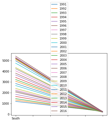
x축에 연도가 와야하므로 전치를 시켜서 다시 그래프를 그려보자.
tdf_ns = df_ns.T
print(tdf_ns.head())
print('\n')

tdf_ns.plot()

     South North
1991  1186   263
1992  1310   247
1993  1444   221
1994  1650   231
1995  1847   230
이번엔 막대 그래프이다. kind='bar' 로 옵션을 설정하면 된다.
tdf_ns.plot(kind='bar')
히스토그램은 kind='hist'로 설정하여 출력한다.
tdf_ns.plot(kind='hist')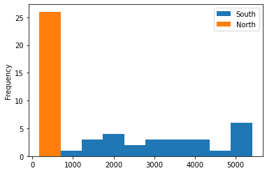
산점도이다.
x축과 y축을 설정하고 kind='scatter'로 설정한다.
df = pd.read_csv('/content/drive/MyDrive/part3/auto-mpg.csv', header=None)

df.columns = ['mpg','cylinders','displacement','horsepower','weight',
              'acceleration','model year','origin','name']
df.plot(x='weight',y='mpg', kind='scatter')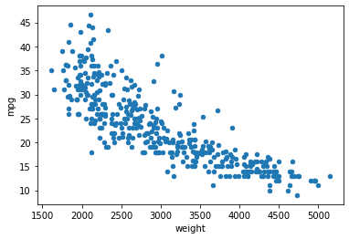
상자그림은 보고 싶은 열을 설정한 후에, kind='box'로 설정한다.
df[['mpg', 'cylinders']].plot(kind='box')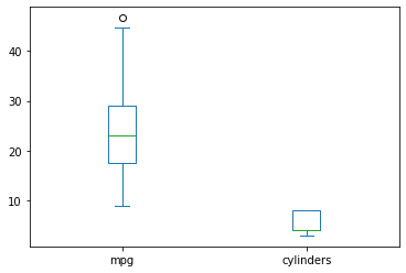
'Study > 혼자 공부하는 판다스' 카테고리의 다른 글
| 혼자 공부하는 판다스 - Seaborn 라이브러리 (0) | 2022.04.21 |
|---|---|
| 혼자 공부하는 판다스 - 시각화 도구 (0) | 2022.04.05 |
| 혼자 공부하는 판다스 - 데이터 저장하기 (0) | 2022.04.04 |
| 혼자 공부하는 판다스 - 외부파일 읽어오기 (0) | 2022.04.04 |
| 혼자 공부하는 판다스 - 인덱스 활용과 산술 연산 (0) | 2022.03.15 |

