데이터를 눈에 보기 쉽게 시각화 전문 도구를 활용하여 시각화 시키는 것이 아주 유리하다.
특히 Matplotlib 은 기본 그래프 도구로 다양한 그래프를 지원하고 있다.
데이터를 다루기 전에는 결측값을 먼저 처리를 해주고나서
그래프를 그리는 등 데이터를 처리 해야 한다.
이를 데이터 전처리라고 하는데, 데이터 전처리에 관해서는 차후에 더 알아보겠다.
import pandas as pd
import matplotlib.pyplot as plt

df = pd.read_excel('/content/drive/MyDrive/part4/시도별 전출입 인구수.xlsx',fillna=0, header=0)
먼저 데이터를 불러오고, matplotlib은 그래프를 그릴 시에 한글 폰트가 깨지는 현상이 나타난다.
깨지지 않도록 코드를 작성해준다.
!sudo apt-get install -y fonts-nanum
!sudo fc-cache -fv
!rm ~/.cache/matplotlib -rf

plt.rc('font', family='NanumBarunGothic')
그리고 데이터를 변경하거나 변형해준다.
df = df.fillna(method = 'ffill') #NaN을 바로 앞 행의 데이터로 채운다.

#서울특별시에서 다른 지역으로 이동한 데이터만 추출
mask = (df['전출지별'] == '서울특별시') & (df['전입지별'] != '서울특별시')
df_seoul = df[mask]
df_seoul = df_seoul.drop(['전출지별'], axis=1)
df_seoul.rename({'전입지별':'전입지'}, axis=1, inplace=True)
df_seoul.set_index('전입지', inplace=True)

#서울에서 경기도로 이동한 인구 데이터 값만 선택한다.
sr_one = df_seoul.loc['경기도']
선 그래프를 그리는 plot() 함수에 x축과 y축 데이터를 선택하면 된다. x축에는 인덱스, y축에 데이터 값
plt.plot(sr_one.index, sr_one.values)
#시리즈 혹은 데이터프레임 객체를 넣어도 가능하다.
plt.plot(sr_one)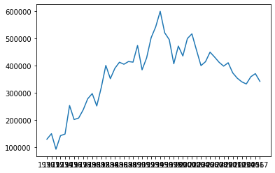
차트의 제목과 축 이름을 추가해보자.
sr_one = df_seoul.loc['경기도']

plt.plot(sr_one.index, sr_one.values)

plt.title('서울 -> 경기 인구 이동')

plt.xlabel('기간')
plt.ylabel('이동 인구수')

plt.show()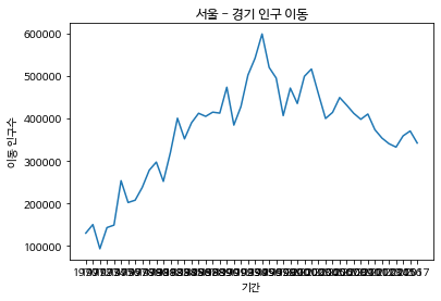
sr_one = df_seoul.loc['경기도']

#그림 사이즈 지정
plt.figure(figsize=(14, 5))
#x축 눈금 라벨 회전
plt.xticks(rotation='vertical')

#x, y축 데이터를 plot 함수에 입력
plt.plot(sr_one.index, sr_one.values)

plt.title('서울-> 경기 인구 이동')
plt.xlabel('기간')
plt.ylabel('이동 인구수')

plt.legend(labels=['서울 -> 경기'], loc='best')
plt.show()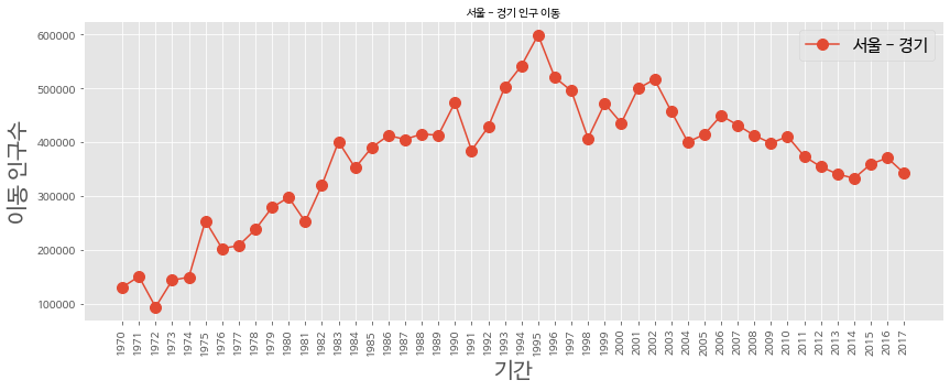
이번에는 그래프에 대한 설명을 덧붙이는 주석을 알아보자.
annotate() 함수를 사용하여 주석 내용을 넣을 위치와 정렬 방법을 지정한다.
글자를 위아래 세로 방향으로 정렬하는 va옵션은 center, top, bottom, baseline 이 있고
좌우 가로 방향으로 정렬하는 ha옵션은 center, left, right가 있다.
plt.style.use('ggplot')

plt.figure(figsize=(14,5))

plt.xticks(size=10, rotation='vertical')

plt.plot(sr_one, marker='o', markersize=10)

plt.title('서울 - 경기 인구 이동', size=10)
plt.xlabel('기간', size=20)
plt.ylabel('이동 인구수', size=20)

plt.legend(labels=['서울 - 경기'], loc='best', fontsize=15)

plt.ylim(50000, 800000)
plt.annotate('', xy=(20, 620000), xytext=(2, 290000), xycoords='data', arrowprops=dict(arrowstyle='->', color='skyblue', lw=5),)

plt.annotate('',
             xy=(47, 450000),
             xytext=(30, 580000),
             xycoords='data',
             arrowprops=dict(arrowstyle='->', color='olive', lw=5),)

plt.annotate('인구 이동 증가(1970-1995)',
             xy=(10, 550000),
             rotation=25,
             va='baseline',
             ha='center',
             fontsize=15,
             )

plt.annotate('인구 이동 감소(1995-2017)',
             xy=(40, 560000),
             rotation=-11,
             va='baseline',
             ha='center',
             fontsize=15,
             )

plt.show()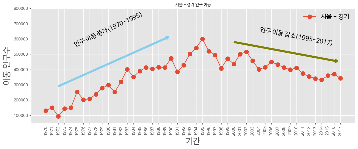
화면을 분할하여 그래프를 여러개 그리는 방법도 있다. add_subplot() 메소드를 적용하여 fig라는
그림틀을 여러개로 분할할 수 있다.
이때 나눠지는 각 부분을 axe 객체라고 부른다.
fig = plt.figure(figsize=(10, 10))
ax1 = fig.add_subplot(2,1,1)
ax2 = fig.add_subplot(2,1,2)

ax1.plot(sr_one, 'o', markersize=10)
ax2.plot(sr_one, marker='o', markerfacecolor='green', markersize=10,
         color='olive', linewidth=2, label='서울->경기')
ax2.legend(loc='best')

ax1.set_ylim(50000, 800000)
ax2.set_ylim(50000, 800000)

ax1.set_xticklabels(sr_one.index, rotation=75)
ax2.set_xticklabels(sr_one.index, rotation=75)

plt.show()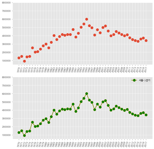
제목과 축 이름을 추가할 수도 있다.
각각 set_xlabel, set_ylabel로 설정 가능하다.
fig = plt.figure(figsize=(20, 5))
ax = fig.add_subplot(1,1,1)

ax.plot(sr_one, marker='o', markerfacecolor='orange', markersize=10,
        color='olive', linewidth=2, label='서울-경기')
ax.legend(loc='best')

ax.set_ylim(50000, 800000)
ax.set_title('서울-경기 인구 이동', size=20)

ax.set_xlabel('기간', size=12)
ax.set_ylabel('이동 인구수', size=12)

ax.set_xticklabels(sr_one.index, rotation=75)

ax.tick_params(axis='x', labelsize=10)
ax.tick_params(axis='y', labelsize=10)

plt.show()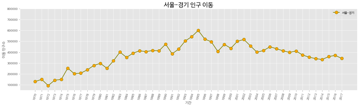
같은 화면에 여러개의 그래프를 추가하는 것도 가능하다.
col_years = list(map(str, range(1970, 2018)))
df_3 = df_seoul.loc[['충청남도', '경상북도','강원도'], col_years]

plt.style.use('ggplot')

fig = plt.figure(figsize=(20, 5))
ax=fig.add_subplot(1,1,1)

ax.plot(col_years, df_3.loc['충청남도',:], marker='o', markerfacecolor='green',
        markersize=10, color='olive', linewidth=2, label='서울 -> 충남')
ax.plot(col_years, df_3.loc['경상북도',:], marker='o', markerfacecolor='blue',
        markersize=10, color='skyblue', linewidth=2, label='서울 -> 경북')
ax.plot(col_years, df_3.loc['강원도',:], marker='o', markerfacecolor='red',
        markersize=10, color='magenta', linewidth=2, label='서울 -> 강원')

ax.legend(loc='best')

ax.set_title('서울 - 충남, 경북, 강원 인구 이동', size=20)

ax.set_xlabel('기간', size=12)
ax.set_ylabel('이동 인구수', size=12)

ax.set_xticklabels(col_years, rotation=90)

ax.tick_params(axis='x', labelsize=10)
ax.tick_params(axis='y', labelsize=10)

plt.show()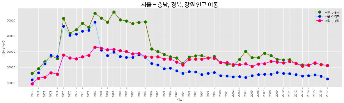
마찬가지로 화면을 4분할하여 그래프를 그릴 수도 있다.
이는 생략하도록 하겠다.
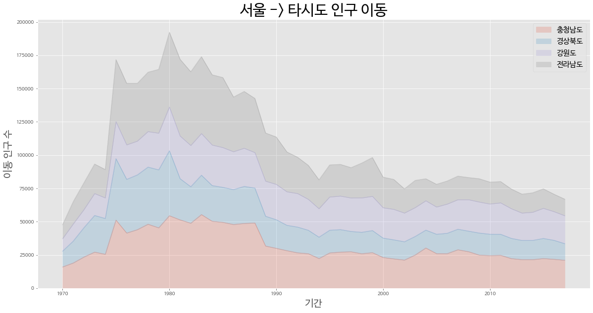
두 번째는 면적 그래프이다. 면적 그래프는 plot() 메소드에 kind='area' 옵션을 추가하면 그릴 수 있다.
mask = (df['전출지별'] == '서울특별시') & (df['전입지별'] != '서울특별시')
df_seoul = df[mask]
df_seoul = df_seoul.drop(['전출지별'], axis=1)
df_seoul.rename({'전입지별':'전입지'}, axis=1, inplace=True)
df_seoul.set_index('전입지', inplace=True)

col_years = list(map(str, range(1970, 2018)))

df_4 = df_seoul.loc[['충청남도', '경상북도', '강원도', '전라남도'], col_years]
df_4 = df_4.transpose()

plt.style.use('ggplot')

df_4.index = df_4.index.map(int)

df_4.plot(kind='area', stacked=False, alpha=0.2, figsize=(20, 10)) #stacked 옵션을 True로
설정하면 선 그래프들이 누적되어서 서로 겹치지 않게 표시 된다.

plt.title('서울 - 타시도 인구 이동', size=10)
plt.ylabel('이동 인구 수', size=20)
plt.xlabel('기간', size=20)
plt.legend(loc='best', fontsize=15)

plt.show()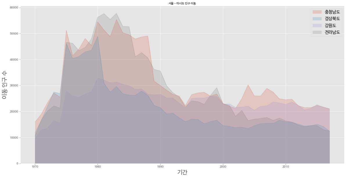
다음은 막대 그래프이다.
plot() 함수에서 kind = 'bar'로 설정하면 막대 그래프를 그릴 수 있다.
col_years = list(map(str, range(2010, 2018)))
df_4 = df_seoul.loc[['충청남도', '경상북도','강원도','전라남도'], col_years]
df_4 = df_4.transpose()

plt.style.use('ggplot')

df_4.index = df_4.index.map(int)

df_4.plot(kind='bar', figsize=(20, 10), width=0.7,
          color = ['orange', 'green', 'skyblue','blue'])

plt.title('서울 -> 타시도 인구 이동', size=30)
plt.ylabel('이동 인구 수', size=20)
plt.xlabel('기간', size=20)
plt.ylim(5000, 30000)
plt.legend(loc='best', fontsize=15)
plt.show()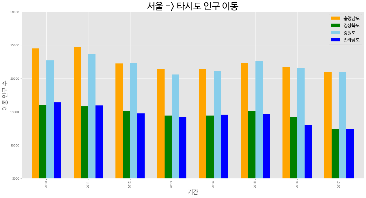
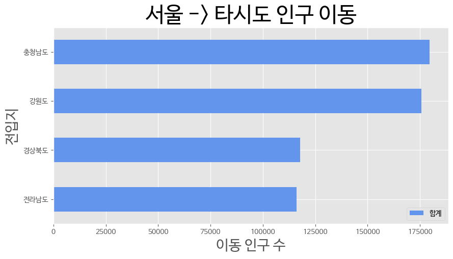
가로형 막대 그래프도 그릴 수 있다. kind='barh'로 설정하면 가능하다.
col_years = list(map(str, range(2010, 2018)))
df_4 = df_seoul.loc[['충청남도', '경상북도','강원도','전라남도'], col_years]

df_4['합계'] = df_4.sum(axis=1)

df_total = df_4[['합계']].sort_values(by='합계', ascending=True)

plt.style.use('ggplot')
df_total.plot(kind='barh', color='cornflowerblue', width=0.5, figsize=(10, 5))

plt.title('서울 -> 타시도 인구 이동', size=30)
plt.ylabel('전입지', size=20)
plt.xlabel('이동 인구 수', size=20)

plt.show()
히스토그램은 kind='hist' 설정하면 그릴 수 있다.
plt.style.use('classic')

df = pd.read_csv('/content/drive/MyDrive/part4/auto-mpg.csv', header=None)

df.columns = ['mpg', 'cylinders', 'displacement', 'horsepower', 'weight',
              'acceleration','model year', 'origin','name']

df['mpg'].plot(kind='hist', bins=10, color='coral', figsize=(10, 5))

plt.title('Histogram')
plt.xlabel('mpg')
plt.show()
산점도는 kind='scatter'로 설정하면 그릴 수 있다.
plt.style.use('default')

df.plot(kind='scatter', x='weight', y='mpg', c='coral', s=10, figsize=(10, 5))
plt.title('Scatter Plot - mpg vs weight')
plt.show()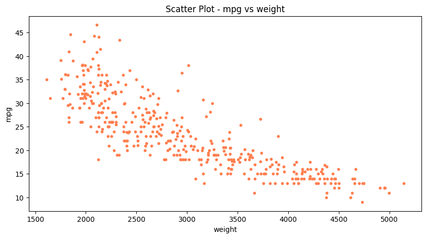
산점도에서 점의 크기를 설정할 수 있다. 이는 새로운 변수를 추가하여 그 변수의 크기만큼으로 크기를 설정
할 수 있는데, 이렇게 표현한 것을 버블 차트라고도 한다.
cylinders_size = df.cylinders/df.cylinders.max() * 300

df.plot(kind='scatter', x='weight', y='mpg', c='coral', figsize=(10,5), s=cylinders_size, alpha=0.3)
plt.title('Scatter Plot : mpg-weight-cylinders')
plt.show()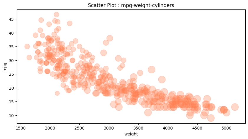
파이 차트는 원을 조각처럼 나누어서 표현한다. kind = 'pie' 옵션을 사용하여 그린다.
df['count'] = 1
df_origin = df.groupby('origin').sum()
print(df_origin.head())

df_origin.index = ['USA', 'EU', 'JPN']

df_origin['count'].plot(kind='pie',
                        figsize=(7, 5),
                        autopct = '%1.1f%%',
                        startangle=10,
                        colors=['chocolate', 'bisque', 'cadetblue'])

plt.title('Model Origin', size=10)
plt.axis('equal')
plt.legend(labels=df_origin.index, loc='upper right')
plt.show()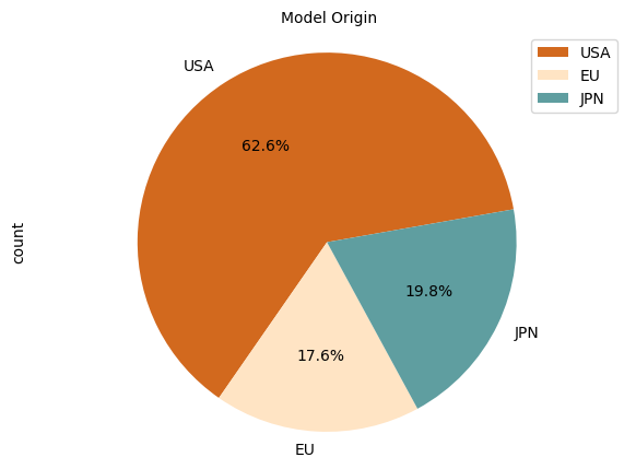
다음은 박스 플롯이다. boxplot() 메소드를 사용하여 그릴 수 있고,
vert=True이면 수직, False이면 수평으로 그릴 수 있다.
fig = plt.figure(figsize=(15, 5))
ax1 = fig.add_subplot(1, 2,1)
ax2 = fig.add_subplot(1,2,2)


ax1.boxplot(x=[df[df['origin']==1]['mpg'],
               df[df['origin']==2]['mpg'],
               df[df['origin']==3]['mpg']],
            labels=['USA', 'EU', 'JAPAN'])
ax2.boxplot(x=[df[df['origin']==1]['mpg'],
               df[df['origin']==2]['mpg'],
               df[df['origin']==3]['mpg']],
            labels=['USA', 'EU', 'JAPAN'],
            vert=False)

ax1.set_title('제조국가별 연비 분포(수직 박스 플롯)')
ax2.set_title('제조국가별 연비 분포(수평 박스 플롯)')

plt.show()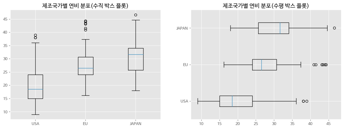
'Study > 혼자 공부하는 판다스' 카테고리의 다른 글
| 혼자 공부하는 판다스 - Folium 라이브러리 (지도 활용) (0) | 2022.04.21 |
|---|---|
| 혼자 공부하는 판다스 - Seaborn 라이브러리 (0) | 2022.04.21 |
| 혼자 공부하는 판다스 - 데이터 살펴보기 (0) | 2022.04.04 |
| 혼자 공부하는 판다스 - 데이터 저장하기 (0) | 2022.04.04 |
| 혼자 공부하는 판다스 - 외부파일 읽어오기 (0) | 2022.04.04 |


